MLE를 활용한 Log-Likelihood Linear Regression 구현 (only numpy)

study/Machine Learning

MLE를 활용한 Log-Likelihood Linear Regression 구현 (only numpy)

ys_cs17 2022. 5. 18. 11:48

Data load를 제외한 모든 Linear Regression의 과정들을 python과 numpy만을 사용하여 구현해보았습니다.

개념에 대한 전체적인 내용은 아래 포스트를 참고하시기 바랍니다.

https://ys-cs17.tistory.com/73

Code implementation

Normalization

weight-height.csv 파일을 DataFrame으로 만든 후 해당 함수를 통해 normalization을 진행합니다.

1. Min max normalization

def min_max_normalize(df):
    x = (df['Weight'] - min(df['Weight'])) / (max(df['Weight']) - min(df['Weight']))
    y = (df['Height'] - min(df['Height'])) / (max(df['Height']) - min(df['Height']))

    return x, y

각 $x, y$에 해당하는 Weight, Height를 min max normalization을 진행합니다.

min max normalization의 수식은 다음과 같습니다.

$$ x_{normalized} = \frac{x - x_{min}}{x_{max}-x_{min}} $$

이는 단순하게 python에서 기본적으로 제공하는 min(), max()를 통해 구현했습니다.

2. z-score normalization

def z_score_norm(df):
    x = (df['Weight'] - df['Weight'].mean()) / df['Weight'].std()
    y = (df['Height'] - df['Height'].mean()) / df['Height'].std()

    return x, y

min max와 동일하게 진행합니다. 수식은 아래와 같습니다.

$$ x_{z-score} = \frac{x - \text{mean}(\bold{x})}{\text{std}(\bold{x})} $$

이 또한 pandas에서 제공하는 mean, std 메서드를 통해 구현을 하였습니다.

Model classes

[1] Gradient 기반 linear regression

class LinearRegression(object):
    def __init__(self, x, y, norm_name):
        self.X = np.array(x).reshape(1, -1)
        self.Y = np.array(y).reshape(1, -1)

        self.num_iteration = 50
        self.N = self.X.shape[1]

        self.weight = np.random.normal(0, 1, (self.X.shape[0], 1))
        self.bias = np.random.rand(1)
        self.step_size = 0.1
        self.norm_name = norm_name

initailize function에 대한 정의는 다음과 같습니다. 데이터 $x,y$를 input으로 받아 reshape 후 저장하고, hyper parameter인 iteration, step size를 지정합니다.

또한 weight와 bias에 대해서도 초기화합니다.

def fit(self):
        for i in range(self.num_iteration):
            self.delta_W = 2 / self.N * (
                np.sum(np.multiply(((np.matmul(self.weight, self.X) + self.bias) - self.Y), self.X)))
            self.deta_bias = 2 / self.N * (np.sum((np.matmul(self.weight, self.X) + self.bias) - self.Y))

            self.weight -= self.step_size * self.delta_W
            self.bias -= self.step_size * self.deta_bias

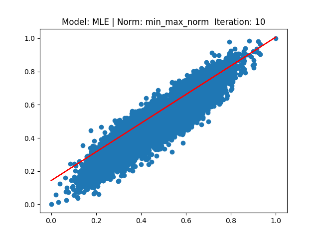
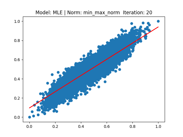
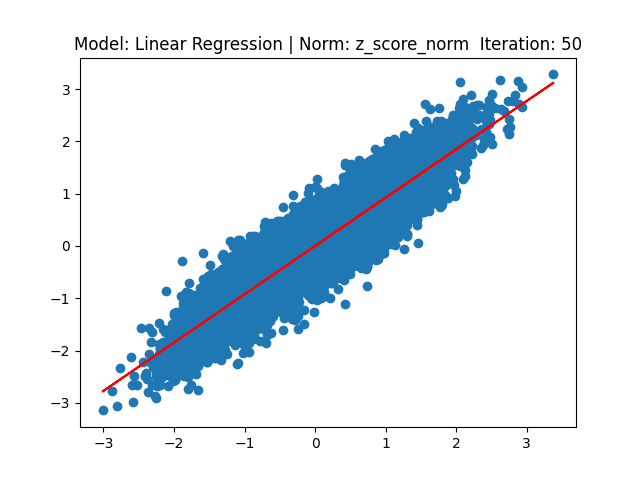
            if (i + 1) % 10 == 0:
                self.show_plot(i)

        return True

학습을 위한 fit 메서드는 다음과 같이 정의하였습니다. weight와 bias에 대한 편미분 값은 수업 시간에 설명한 수식과 같이 정의하였습니다.

$$ \text{delta} \ w = \frac{2}{N} \sum_{i=1}^{N}(wx_{i} + b - y_{i}^{true}) \cdot x_{i} $$

$$ \text{delta }b = \frac{2}{N}\sum_{i = 1}^{N}({w}x_{i}+b - y_{i}^{true}) $$

해당 gradient와 step size를 곱해줌으로서 wieght 및 bias를 갱신합니다.

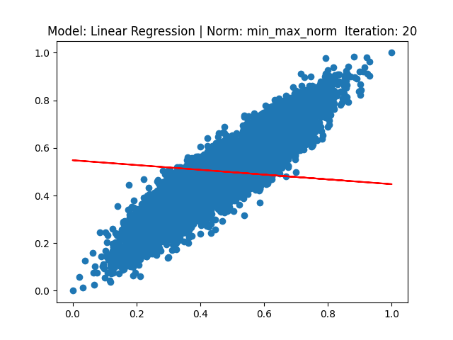
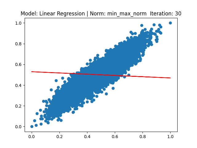
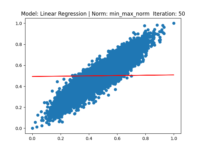
또한 10 iter 마다 1번씩 plot을 그립니다. show_plot() 메서드는 잠시 후에 설명드리겠습니다.

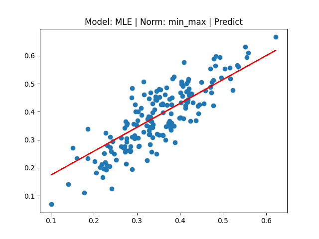
def predict(self, X):
        product = np.matmul(self.weight, np.array(X).reshape(1, -1)) + self.bias

        return product.reshape(-1)

test를 위한 predict 메서드는 다음과 같이 정의했습니다. input으로 test dataset을 받고, 이를 line equation을 통해 예측을 수행합니다. 수식은 다음과 같습니다.

$$ y_{i}^{pred} = wx_{i} + b $$

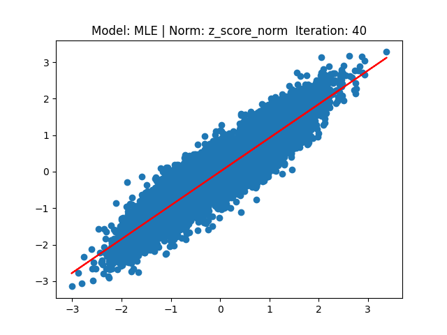
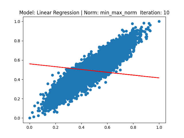
def show_plot(self, iter):
        plt.title('Model: Linear Regression | Norm: {}  Iteration: {}'.format(self.norm_name, iter + 1))
        plt.scatter(self.X, self.Y)
        plt.plot(self.X.squeeze(), self.predict(self.X), 'red')
        # plt.show()
        plt.savefig("result_plot/regression_{}_{}".format(self.norm_name, iter + 1))
        plt.close()

show_plot 메서드는 위 코드와 같습니다.

기존 train dataset의 x, y를 scatter를 통해 그리고, step 10마다 pred 메서드를 통해 나온 $\hat{y}$를 통해 직선으로 그린 후 저장 또는 화면에 표출합니다.

[2] MLE 기반 linear regression

class MLE(object):
    def __init__(self, x, y, norm_name):
        self.X = np.array(x).reshape(1, -1)
        self.Y = np.array(y).reshape(1, -1)
        self.num_iteration = 50

        self.N = self.X.shape[1]

        self.weight = np.random.normal(0, 1, (self.X.shape[0], 1))
        self.bias = np.random.rand(1)
        self.step_size = 0.1
        self.norm_name = norm_name

MLE class의 initialize function은 LinearRegression class와 동일합니다.

def fit(self):
    for i in range(self.num_iteration):
        delta_w, delta_b = self.grad()

        self.weight -= self.step_size * delta_w
        self.bias -= self.step_size * delta_b

        if (i + 1) % 10 == 0:
            self.show_plot(i)

    return True

fit 메서드도 이전 class와 동일합니다. grad 메서드를 통해 delta_w, delta_b 값을 return 받습니다.

def grad(self):
        delta_w = (-2 / self.N) * (np.sum(np.multiply((self.Y - (np.matmul(self.weight, self.X) + self.bias)), self.X)))
        delta_b = (-2 / self.N) * (np.sum((self.Y - (np.matmul(self.weight, self.X) + self.bias))))

        return delta_w, delta_b

grad 메서드는 다음과 같이 구현하였습니다. 이전 gradient 기반과 비슷해 보이지만 수식적으로는 약간의 차이가 있습니다.

MLE 수식을 계산하기 위해 weight를 추정하는 통계적 수식은 다음과 같이 정의할 수 있습니다.

$$ \hat{\theta} = \argmax_{\theta}{\log{p(\mathcal{D} \mid \theta)}} $$

식을 간략하게 설명하면 train data와 weight 간 최적화하는 지점을 찾는 것입니다. 이는 로그를 써서 최대화할 수 있는 $\theta$인 weight 값을 찾는 것이 MLE의 목표입니다.

위 수식에서 $\mathcal{D}$는 train dataset을 의미하고, 이는 $\mathcal{D} = \left\{ x_{1}, \dots, x_{n} \right\}$로 정의됩니다. $\mathcal{D}$ 가 $\text{i.i.d.}$를 만족한다면 Log-likelihood의 식을 다음과 같이 정의할 수 있습니다.

$$ \mathcal{l}= \log{p(\mathcal{D} \mid \theta)} = \sum_{i = 1}^{N}{\log{(y_{i} \mid x_{i}, \theta})} $$

Log likeli-hood를 최대화 하는 것과 $\text{NLL}$ (Negative log likeli-hood)를 최소화하는 것이 같다는 것을 알 수 있습니다. NLL의 수식은 다음과 같습니다.

$$ \text{NLL}(\theta) = -\sum_{i = 1}^{N}{\log{(y_{i} \mid x_{i}, \theta})} $$

NLL은 Log likeli-hood에 -를 붙인 것과 같습니다. Maximum 하는 문제보다는 Minimum 하는 문제가 software optimization 측면에서는 때때로 더 편리하기 때문에 $\text{NLL}$을 사용합니다.

위에서 구한 수식을 활용하여 MLE의 적용을 하면 식은 다음과 같이 정의할 수 있습니다.

$$ \mathcal{l}(\theta) = \sum_{i=1}^{N}{\log{\left[\left(\frac{1}{2\pi \sigma^{2}}\right)^{\frac{1}{2}}\text{exp}{\left(-\frac{1}{2\sigma^{2}}\left(y_{i}- w^{T}x_{i}\right)\right)^{2}}\right]}} \\ = -\frac{1}{2}\text{RSS}(w) - \frac{N}{2}\log(2\pi \sigma^{2}) $$

여기서 RSS는 다음과 같이 정의됩니다.

$$ \text{RSS}(w) = \sum_{i =1}^{N}(y_{i} - w^{T}x_{i})^{2} $$

$\sum$안에 존재하는 식들이 residual error입니다. 이는 정답 label $y$ 에 대한 input vector $x$ 와 weight인 $w$에 대한 차의 제곱입니다. optimization을 위해 residual error를 최소화해야 하는데, 이들의 합에 대해 최소화를 진행합니다. $\text{RSS}$는 $\text{SSE}$(sum of squared error)라고도 불리는데, 이를 data size인 $N$ 만큼 나누게 된다면 $MSE$ 수식이 됩니다. 이를 통해 $\text{RSS}$를 최소화하여 $w$에 대한 $\text{MLE}$ 수식을 구해야 하고, 이를 least squares라고 부릅니다.

$$ \text{RSS}(w) = \sum_{i=1}^{N}(y_{i}- (w^{T}x_{i}+b))^{2} $$

이번 프로젝트에서 사용하는 실질적인 수식은 위와 같습니다.

다른 상수들은 $w$와 $b$에 영향을 받지 않기 때문에 제외하고 이에 대해 편미분을 하면 식은 다음과 같아집니다.

$$ \text{delta }w= -2(y-(ax+b))x $$

$$ \text{delta }b= -2(y-(ax+b)) $$

이렇게 구한 gradient를 가지고 weigth 및 bias에 대한 갱신을 진행합니다.

predict, show_plot 메서드는 이전 class와 같아 설명을 생략합니다.

main code

import numpy as np
import matplotlib.pyplot as plt
import pandas as pd

from model import LinearRegression, MLE
from preprocess import min_max_normalize, z_score_norm

np.warnings.filterwarnings('ignore', category=np.VisibleDeprecationWarning)

numpy, matplotlib, pandas를 import 해주고, 지금까지 설명드린 normalization, model에 대한 함수 및 class도 import 해줍니다.

if __name__ == "__main__":
    data = pd.read_csv("./dataset/weight-height.csv")
    df = pd.DataFrame(data)

    # ----------------Model: MLE, Norm: z_score----------------
    x, y = z_score_norm(df)

    MLE_reg_z_norm = MLE(x[:-180], y[:-180], "z_score_norm")

    if MLE_reg_z_norm.fit():
        print("MLE z_norm Fitting finish")

    else:
        print("Error")

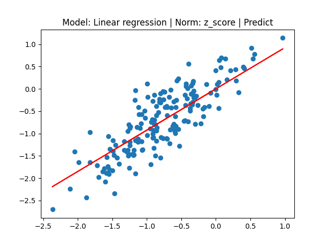
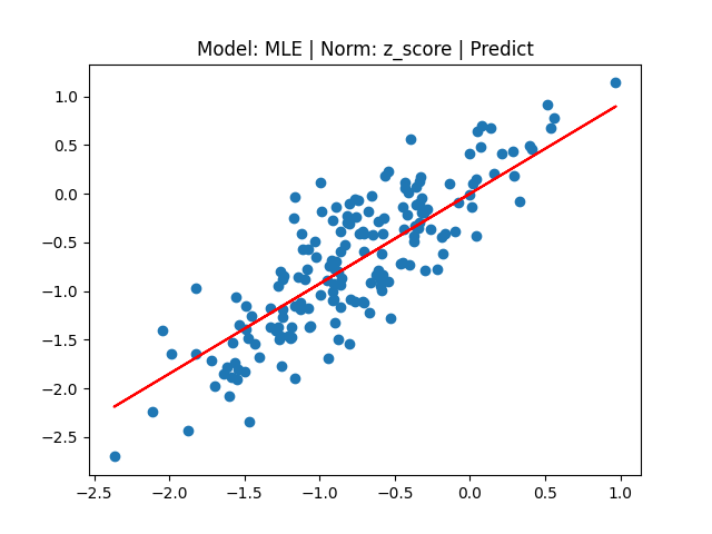
    MLE_pred = MLE_reg_z_norm.predict(np.array(x[-180:]))

    plt.title("Model: MLE | Norm: z_score | Predict")
    plt.scatter(x[-180:], y[-180:])
    plt.plot(x[-180:], MLE_pred, 'red')

    # plt.show()

    plt.savefig("result_plot/result_MLE_z_score_norm")
    plt.close()

주어진 데이터를 pandas로 읽고, 이를 구현 용이를 위해 DataFrame으로 변경합니다. 그 후 z-score 또는 min max normalization을 진행한 후 model class를 생성해줍니다.

이후 fit과 predict를 진행한 후 최종적인 결과를 plot화 합니다.

총 4가지 (model 2가지, normalization 2가지) 방법을 main에 구현하였습니다. 각 class 및 normalization 호출만 다르고 나머지 코드는 같아 설명은 생략하겠습니다.